Designing Diffusion Models in Real World
A review of a paper, Elucidating the Design Space of Diffusion-Based Generative Models. This post focuses on the reasons of the engineering details in the paper.
Overview
In deep learning, practical implementations are just as important as theoretical supports. Especially when proposing new paradigms, such as GANs, diffusion models, and transformers, etc., engineering skills are essential to bring the paradigms into the real world. Even if the suggested designs on diffusion models in Elucidating the Design Space of Diffusion-Based Generative Models (EDM)
Revisit Diffusion Models
Reformulate diffusion models
Score-Based Model
where \(p(\mathrm{x};\sigma) = \left[p_{\text{data}} * \mathcal{N}(\mathrm{0}, \sigma^2\mathrm{I})\right](\mathrm{x})\).
Then, the corresponding probability flow ODE is
\[\begin{align} d\mathrm{x} = \left[\dot{s}(t)/s(t) - s(t)^2 \dot{\sigma}(t)\sigma(t) \nabla_\mathrm{x} \log p(\mathrm{x}_t/s(t);\sigma(t)) \right] dt. \label{edm:ode} \end{align}\]Obstacles in diffusion models
Generation by diffusion models can interpreted as solving ODE:
\[\begin{align} d\mathrm{x} = f(\mathrm{x}_t, s(t), \sigma(t))dt. \end{align}\]-
\(f(\mathrm{x}_t, s(t), \sigma(t))\) is not known and it is parametrized by a network \(f_\theta(\mathrm{x}_t, s(t), \sigma(t))\). The inaccurate approximation on the target causes degradation.
→ Better training! -
The solution at \(t=0\) given boundary condition at \(t=T\) is
\(\begin{align} \mathrm{x}_0 = \mathrm{x}_T + \int_0^T f(\mathrm{x}_t, s(t), \sigma(t))dt. \end{align}\) The integral is numerically calculated, which causes truncation errors.
→ Reduce truncation errors, focus on important region!
Design space of diffusion models
Components regarding training
- Parametrization and network preconditioning: \(c_\text{skip}(\sigma)\), \(c_\text{out}(\sigma)\), \(c_\text{in}(\sigma)\), \(c_\text{noise}(\sigma)\).
- Loss weighting: \(\lambda(t)\).
- Noise level distribution for training: \(\sigma \sim p_{\text{noise}}\).
- Augmentation
Components regarding deterministic sampling
- Truncation-error-reducing ODE: \(s(t)\), \(\sigma(t)\).
- Truncation-error-reducing algorithms: Higher-roder integrators
- Distributing truncation errors properly: Discretization \(\{t_i\}_0^N\)
Components regarding stochastic sampling
- Rate of replaced noises: \(\beta(t)\)
- Heuristics: \(S_{\text{tmin}}, S_{\text{tmax}}, S_{\text{noise}}, S_{\text{churn}}\).
Improvements to Training
For this section, this post assumes \(s(t)=1\).
Parametrization, network preconditioning, loss weighting
\(D(\mathrm{x}_t,\sigma)\) is a denoiser which minimizes \(\ell_2\)-norm with \(\mathrm{y}\): \(\begin{align} \mathbb{E}_{\mathrm{y} \sim p_{\text{data}}} \mathbb{E}||D(\mathrm{y} + \mathrm{n}) - \mathrm{y}||_2^2. \label{eq:loss} \end{align}\)
Then, the relation between a score function and the ideal denoiser is \(\begin{align} \nabla_{\mathrm{x}} \log p(\mathrm{x};\sigma) = (D(\mathrm{x};\sigma) - \mathrm{x}) / \sigma^2. \end{align}\)
Networks in many baselines predicts either \(D(\mathrm{x},\sigma)\) or \(\mathrm{n}\). However, Dynamic dual-output diffusion models
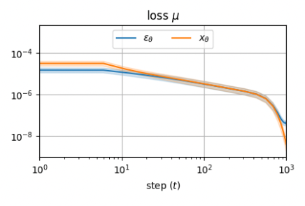 |
|---|
| Loss comparison between predicting the denoised output or the added noise. |
From the observation, EDM
Then the loss function (\ref{eq:loss}) is \(\begin{align} \mathbb{E}_{\sigma,\mathrm{y},\mathbf{b}}\left[ \underbrace{\lambda(\sigma)c_{\text{out}}(\sigma)^2}_{\text{effective weight}} ||\underbrace{F_\theta(c_{\text{in}}(\sigma)(\mathrm{y}+\mathbf{n};c_{\text{noise}}(\sigma)))}_{\text{network output}} - \underbrace{\frac{1}{c_{\text{out}}(\sigma)}(\mathrm{y} - c_{\text{skip}}(\sigma)(\mathrm{y}+\textbf{n}))}_{\text{effective training target}}||_2^2 \right]. \end{align}\)
1.Network inputs should have bounded range
\(\begin{align} \Rightarrow &\text{Var}_{\mathrm{y},\mathbf{n}}\left[c_{\text{in}}(\sigma)(\mathrm{y} + \mathbf{n})\right] = 1 \\ \Rightarrow &c_{\text{in}}(\sigma) = 1 / \sqrt{\sigma^2 + \sigma_{\text{data}}^2}\\ \text{& } &c_{\text{noise}}(\sigma) = \log (\sigma)/4 \end{align}\)
2.Effective training target should have bounded range
\(\begin{align} &\Rightarrow \text{Var}_{\mathrm{y},\mathbf{n}}\left[\frac{1}{c_{\text{out}}(\sigma)}(\mathrm{y} - c_{\text{skip}}(\sigma)(\mathrm{y}+\textbf{n}))\right] = 1 \\ &\Rightarrow c_{\text{out}}(\sigma)^2 = (1-c_{\text{skip}}(\sigma))^2\sigma_{\text{data}}^2 + c_{\text{skip}}(\sigma)^2 \sigma^2 \end{align}\)
3.Errors of network should not be amplified
\(\begin{align} \Rightarrow~ &c_{\text{skip}}(\sigma) = \underset{c_{\text{skip}}(\sigma)}{\text{argmin}} ~c_{\text{out}}(\sigma) \\ \Rightarrow~ &\begin{cases} c_{\text{skip}}(\sigma) = \sigma_{\text{data}}^2 / (\sigma^2 + \sigma_{\text{data}}^2) \\ c_{\text{out}}(\sigma) = \sigma \cdot \sigma_{\text{data}} / \sqrt{\sigma^2 + \sigma_{\text{data}}^2} \end{cases} \end{align}\)
4. Effecitve weight should be uniform
\(\begin{align} \Rightarrow~ &\lambda(\sigma)c_{\text{out}}(\sigma)^2 = 1 \\ \Rightarrow~ & \lambda(\sigma) = (\sigma^2 + \sigma_{\text{data}}^2)/(\sigma \cdot \sigma_{\text{data}})^2 \end{align}\)
Putting 1 ~ 4 together, the expected value of the loss at each noise level is 1. Moreover, the change of effective training target according to \(\sigma\) coincides to the observation of Dynamic dual-output diffusion models
Noise level distribution for training
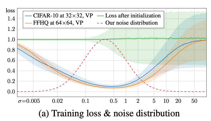 |
|---|
| Observed loss per noise level. The shaded regions represent the standard deviation over 10k random samples. EDM’s proposed training sample density is shown by the dashed red curve. |
At low noise levels, seperating the small noise components is difficult and irrelevant, whereas at high noise levels, the correct answer approaches to dataset average; EDM
Augmentataion
EDM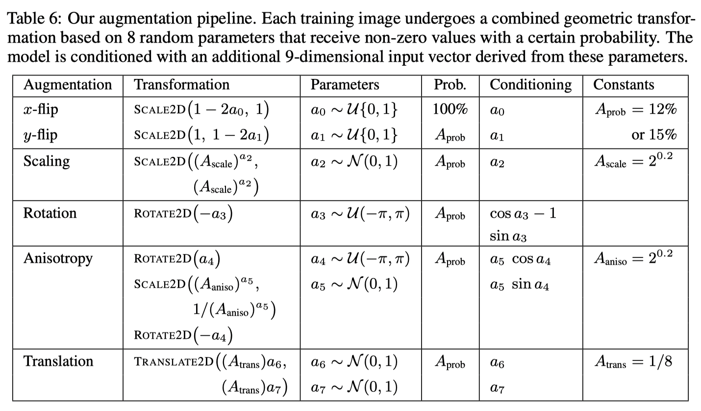
- Each agmentation is enabled with \(A_{\text{prob}}\).
- Draw \(a_i\) from each enabled augmentation and construct transformation matrix.
- Pass data through \(2\times\) supersampled high-quality Wavelet filters.
- Construct a 9-dimensional conditioning input vector for non-leaking augmentation. This vector makes the network to perform auxiliarty tasks.
Improvements to Deterministic Sampling
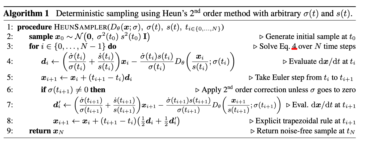
Higher-order integrators
For \(s(t)=1\) and \(\sigma(t)=t\), the ODE to solve is
\[\begin{align} d\mathrm{x}/dt = (\mathrm{x}_t - D(\mathrm{x}_t;t))/t := f(\mathrm{x}_t,t). \end{align}\]Euler method
Euler method approximates the integral by
\[\begin{align} \int_{t_{i}}^{t_{i-1}} f(\mathrm{x}_t,t) dt = (t_{i-1} - t_{i})f(\mathrm{x}_{t_i},t_i) + O(|t_{i-1}-t_{i}|^2). \end{align}\]Therefore, the total truncation error is \(O(\max \lvert t_{i-1}-t_{i} \rvert)\). Let \(\hat{\mathrm{x}}_{t_{i-1}}\) is a solution obtained by Euler method.
Heun’s method
Then, Heun’s method approximates the integral by
\[\begin{align} \int_{t_{i}}^{t_{i-1}} f(\mathrm{x}_t,t) dt = (t_{i-1} - t_{i})(f(\mathrm{x}_{t_i},t_i)+ f(\hat{\mathrm{x}}_{t_{i-1}},t_{i-1}))/2+ O(|t_{i-1}-t_{i}|^3). \end{align}\]Therefore, the total truncation error is \(O(\max{\lvert t_{i-1}-t_{i}|^2 \rvert})\). Huen’s method decreases truncation error at the cost of one additional evaluation of the network.
Deterministic sampling algorithm for EDM
Discretization
As long as using numerical integrators with limited computational resources, truncation errors are inevitable. In terms of obtaining ODE trajectories accurately, it is important to minimize total truncation erros. Hoever, the interests of diffusion models at generation are only the solutions at low noise levels; it is reasonable to focus on low noise levels. EDM discretizes as
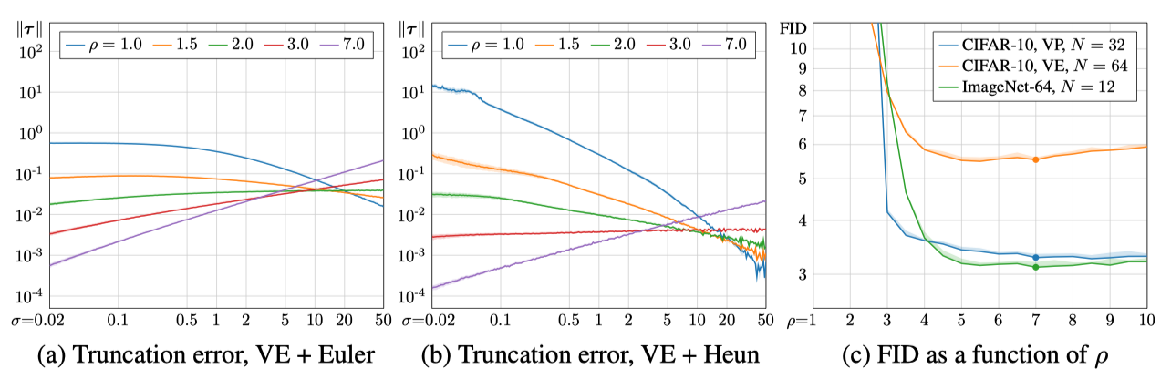
\[\begin{align} t_{N-i} = \sigma_{i< N} = (\sigma_{\text{max}}^{1/\rho} + \frac{i}{N-1} (\sigma_{\text{min}}^{1/\rho} - \sigma_{\text{max}}^{1/\rho}))^\rho, \sigma_N = 0. \end{align}\]Increasing \(\rho\) results dense discretizations at low noise levels.
 |
|---|
| (a),(b) Local truncation error at different noise levels. (c) FID as a function of \(\rho\). |
\(\rho=3\) nearly equalizes the truncation error at each step as in (a), (b). On the other hand, \(\rho=7\) generates better samples as in (c). Proper value of \(\rho\) changes according to the tasks. e.g., equalized truncation error will be better for solving ODE in both directions.
Truncation-error-reducing ODE
Many integrators including Euler and Heun’s method have small truncation errors if \(f(\mathrm{x}_t,t)\) has small curvature, or is close to linear function. \(s(t)\) and \(\sigma(t)\) determine the shape of the ODE solution trajectories, which is closely related to linearity of the \(f(\cdot)\).
\[\int_{t_{i}}^{t_{i-1}} f(\mathrm{x}_t,t) dt \approx \begin{cases} (t_{i-1} - t_{i})f(\mathrm{x}_{t_i},t_i) & \text{Euler method} \\ (t_{i-1} - t_{i}) (f(\mathrm{x}_{t_i},t_i)+ f(\hat{\mathrm{x}}_{t_{i-1}},t_{i-1}))/2 & \text{Heun's method} \end{cases}\]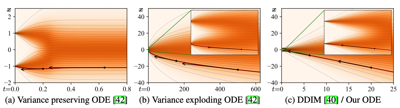 |
|---|
| A sketch of ODE curvature in 1D where \(p_{\text{data}}\) is two Dirac peaks at \(\mathrm{x}= \pm 1\). Axis is chosen to show \(\sigma \in [0,25]\) and zoom in \(\sigma \in [0,1]\). (c) sketches the curvature when \(s(t)=1\) and \(\sigma(t)=t\). It has small curvature, while the tangent directs to the datapoints. |
Results of deterministic sampling
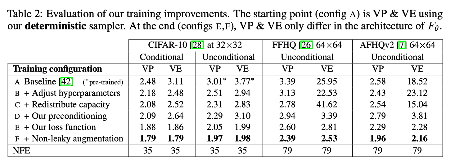
- Config B changes basic hyperparameters such as batch size, learning rate, dropout, etc; it disable gradient clipping
- Config C improves the expressive power of the model.
- Configs D, E, and F are explained in the previous context.
Stochastic Sampling
SDE formulation
EDM
Role of stochasticity
In theory, ODE and SDE have the same marginal distributions. However in practice, stochasticity in sampling often enhances the sample quality. The authors attribute the beneficial role of stochasticity to the following steps:
- \(\mathrm{x}_t\) deviates from the ideal marginal distribution, due to the training and truncation errors.
- The Langevin diffusion drives the sample towards the ideal marginal distribution.
Stochastic sampling algorithm in EDM
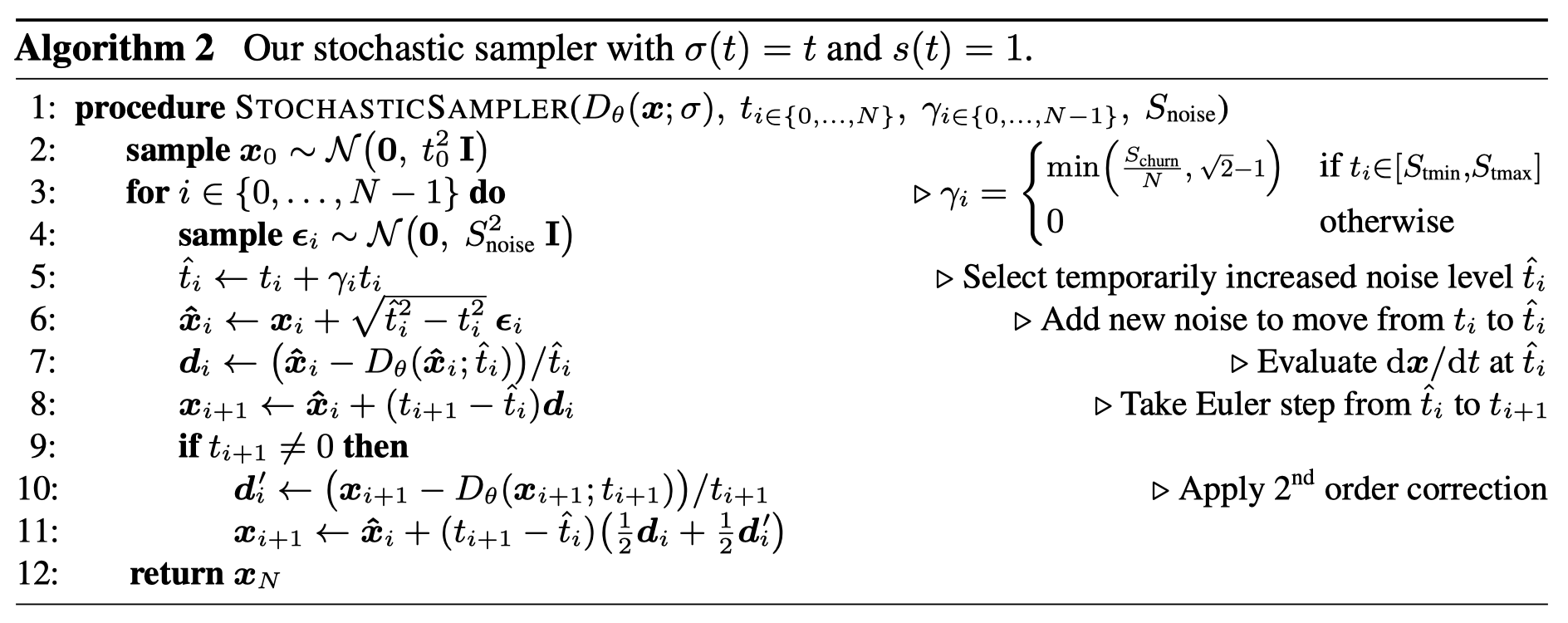
Stochastic sampling algorithm in EDM
- Noise injection: integrate noise into samples according to \(\gamma_i \geq 0\).
- Noise decay with probability flow: solve the ODE from increased noise level to desired level.
Algorithm in real world
 |
|---|
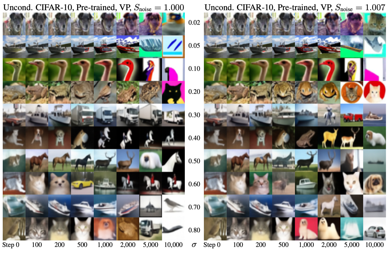
| Observe the effect of Langevin diffusion in real world: there is gradual image degradation with the repeated addition and removal of noise. A random image is drawn from \(p(\mathrm{x};\sigma)\) and Algorithm 2 is run for a certain number of steps with \(\gamma_i=\sqrt{2}-1\). |
Langevin diffusion is supposed to drive the sample towards the true data distribution, however…
- For low noise levels, images drift toward oversaturated colors.
- For high noise levels, images become abstract when \(s_{\text{noise}}=1\).
Authors suspect that non-conservative vector field generated by parametrized denoiser violates the premises of Langevin diffusion since their analytical denoisers have not shown such degradation.
\(\Rightarrow\) Fix flaws of \(D_\theta(\mathrm{x};\sigma)\) with heuristics!
-
For low noise levels, images drift toward oversaturated colors.
\(\Rightarrow\) Enable stochasticity within \(t_i \in [S_{\text{tmin}}, \underline{S_{\text{tmax}}}]\). -
For high noise levels, images become abstract when \(S_{\text{noise}}=1\).
\(\Rightarrow\) \(D_\theta(\cdot)\) removes too much noise because of regression towards the mean, which often happens when \(\ell_2\) trained.
\(\Rightarrow\) Inflate the standard deviation of newly added noise: \(S_{\text{noise}}>1\). -
New noise never exceeds the noise already in the image.
\(\Rightarrow\) Clamp \(\gamma_i\). -
Controls the overal stochasticity by \(S_{\text{churn}}\).
Results of stochastic sampling
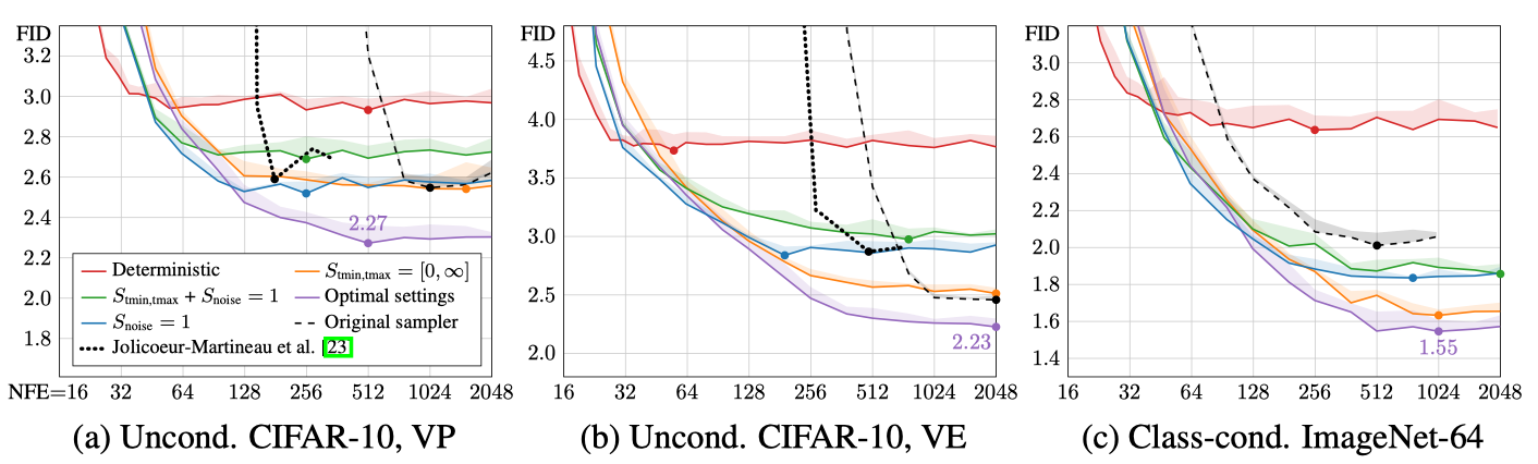 |
|---|
| Evaluation of stochastic samplers with ablations. Red line is deterministic sampler while purple line is optimal stochastic sampler. |