Understanding Diffusion Models in Two Perspectives

A review of two papers, Denoising diffusion probabilistic models and Score-Based Generative Modeling through Stochastic Differential Equations. This post focuses on theoretical backgrounds of diffusion models, rather than implementations.

Overview

DDPM and Score-Based Model introduce diffusion model as a new paradigm of generative models. Since the concepts of both papers are similar, one might regard Score-Based Model as only a continuous version of DDPM. Two papers have slight different views, even their loss functions and implementations are similar.

This post mainly explains how formulations and objectives of two papers are different, and how they are related even with the differences.

Summary of the post

The objective of DDPM is to minimize the surrogate of the negative log-likelihood.
The objective of Score-Based Model is to match marginal distributions of forward SDE and backward SDE/ODE.
Even with the differences, both derivations require the score function, differential of the log of the probability density function. The score functions are parametrized by neural networks and both papaers have similar loss functions.

Maximizing Log-Likelihood

Forward (Diffusion) Process

The forward process is a Markov chain that gradually adds Gaussian noise to the data for \(T\) steps with distributions defined as follows: \(\begin{align} &\mathrm{x}_t \perp\mkern-9.5mu\perp \mathrm{x}_{0:t-1}, \\ &q(\mathrm{x}_0) := \mathrm{P}_{data}(\mathrm{x}_0), \\ &q(\mathrm{x}_t|\mathrm{x}_{t-1}) := \mathcal{N}(\mathrm{x}_t;\sqrt{1-\beta_t}\mathrm{x}_{t-1}, \beta_t \mathrm{I}), \end{align}\)

where \(\{\beta_t\}_{t=1}^T\) are pre-defined constants.

Backward (Denoising) Process

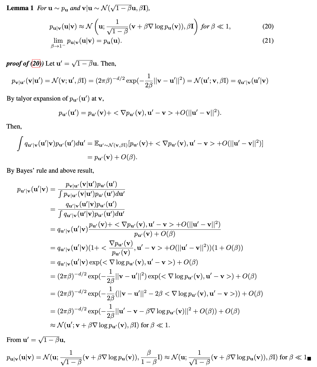
The backward process is a Markov chain that gradually denoises perturbed data and it is parametrized by neural networks. When \(\beta_t\ll 1\) the backward distribution can be approximated as \(\begin{align} q(\mathrm{x}_{t-1}|\mathrm{x}_{t}) \approx \mathcal{N}(\mathrm{x}_{t-1}; \cfrac{1}{ \sqrt{1-\beta_t}}(\mathrm{x}_{t} + \beta_t \nabla \log q (\mathrm{x}_t)), \beta_t \mathrm{I}). \end{align}\)

proof.

It is reasonable to parametrize the denoising distribution as Gaussian as long as \(\{\beta_t\}_{t=1}^T\) are infinitesimal. Therefore the bacward process is defined as follows: \(\begin{align} &\mathrm{x}_t \perp\mkern-9.5mu\perp \mathrm{x}_{t+1:T}, \\ &p(\mathrm{x}_T) := \mathcal{N}(\mathrm{x}_T; \mathrm{0}, \mathrm{I}) \\ &p(\mathrm{x}_{t-1}|\mathrm{x}_{t}) = \mathcal{N}(\mathrm{x}_{t-1}; \cfrac{1}{ \sqrt{1-\beta_t}}(\mathrm{x}_{t} + \beta_t s_\theta(\mathrm{x}_t,t)), \beta_t \mathrm{I}), \end{align}\)

Note that we expect \(s_\theta(\mathrm{x}_t,t)\) to learn \(\nabla\log q(\mathrm{x}_t)\).

Minimizing Surrogate of Negative Log-Likelihood

The negative log-likelihood of data is \(\begin{align} \mathbb{E}_{\mathrm{x}_0 \sim q} \left[-\log p(\mathrm{x}_0)\right] &\leq \mathbb{E}_{\mathrm{x}_0 \sim q} \mathbb{E}_{\mathrm{x}_{1:T|0} \sim q} \left[ \log \cfrac{q(\mathrm{x}_{1:T}|\mathrm{x}_{0})}{p(\mathrm{x}_{0:T})} \right]. \end{align}\)

proof.

\[\begin{align*} -\log p(\mathrm{x}_0) &= -\log \int p(\mathrm{x}_{0:T}) d\mathrm{x}_{1:T} \\ &= -\log \int q(\mathrm{x}_{1:T}|\mathrm{x}_{0}) \cfrac{p(\mathrm{x}_{0:T})}{q(\mathrm{x}_{1:T}|\mathrm{x}_{0})} d\mathrm{x}_{1:T} \\ &\leq -\int q(\mathrm{x}_{1:T}|\mathrm{x}_{0}) \log \cfrac{p(\mathrm{x}_{0:T})}{q(\mathrm{x}_{1:T}|\mathrm{x}_{0})} d\mathrm{x}_{1:T} ~~(\because \text{Jensen})\\ &= \mathbb{E}_{\mathrm{x}_{1:T|0} \sim q} \left[ \log \cfrac{q(\mathrm{x}_{1:T}|\mathrm{x}_{0})}{p(\mathrm{x}_{0:T})} \right]. \end{align*}\]

Using Markov properties, \(\begin{align} &q(\mathrm{x}_{1:T} | \mathrm{x}_0) = q(\mathrm{x}_T | \mathrm{x}_0) \prod_{t=2}^T q(\mathrm{x}_{t-1} | \mathrm{x}_t, \mathrm{x}_0), \\ &p(\mathrm{x}_{T:0}) = p(\mathrm{x}_T) \prod_{t=T}^{1} p(\mathrm{x}_{t-1}|\mathrm{x}_t). \end{align}\)

proof.

\[\begin{align*} q(\mathrm{x}_{1:T} | \mathrm{x}_0) &= \prod_{t=1}^{T} q(\mathrm{x}_{t}|\mathrm{x}_{0:t-1}) \\ &= \prod_{t=1}^{T} q(\mathrm{x}_{t}|\mathrm{x}_{t-1}) \\ &= q(\mathrm{x}_1|\mathrm{x}_0)\prod_{t=2}^{T} q(\mathrm{x}_{t}|\mathrm{x}_{t-1}, \mathrm{x}_{0}) \\ &= q(\mathrm{x}_1|\mathrm{x}_0)\prod_{t=2}^{T} \frac{q(\mathrm{x}_{t},\mathrm{x}_{t-1}| \mathrm{x}_{0})}{q(\mathrm{x}_{t-1}| \mathrm{x}_{0})} \\ &= q(\mathrm{x}_1|\mathrm{x}_0)\prod_{t=2}^{T} \frac{q(\mathrm{x}_{t}|\mathrm{x}_{0})q(\mathrm{x}_{t-1}| \mathrm{x}_{t},\mathrm{x}_{0})}{q(\mathrm{x}_{t-1}| \mathrm{x}_{0})} \\ &= q(\mathrm{x}_T | \mathrm{x}_0) \prod_{t=2}^T q(\mathrm{x}_{t-1} | \mathrm{x}_t, \mathrm{x}_0), \\ p(\mathrm{x}_{T:0}) &= p(\mathrm{x}_T) \prod_{t=T}^{1} p(\mathrm{x}_{t-1}|\mathrm{x}_{T:t})\\ &= p(\mathrm{x}_T) \prod_{t=T}^{1} p(\mathrm{x}_{t-1}|\mathrm{x}_t). \end{align*}\]

Therefore, the surrogate of negative log-likelihood becomes \(\begin{align} &D_{KL}(q(\mathrm{x}_T|\mathrm{x}_0) || p(\mathrm{x}_T)) + \mathbb{E}_q\left[-\log p(\mathrm{x}_0|\mathrm{x}_1)\right] \nonumber \\ &+ \sum_{t=2}^T D_{KL}(q(\mathrm{x}_{t-1} | \mathrm{x}_t, \mathrm{x}_0) || p(\mathrm{x}_{t-1}|\mathrm{x}_t)). \end{align}\)

The surrogate of negative log-likelihood can be explictly expressed using \(\begin{align} &p(\mathrm{x}_{t-1}|\mathrm{x}_{t}) = \mathcal{N}(\mathrm{x}_{t-1}; \cfrac{1}{ \sqrt{1-\beta_t}}(\mathrm{x}_{t} + \beta_t s_\theta(\mathrm{x}_t,t)), \beta_t \mathrm{I}), \\ &q(\mathrm{x}_{t-1}|\mathrm{x}_{t}, \mathrm{x}_{0}) = \mathcal{N}(\mathrm{x}_{t-1}; \cfrac{1}{ \sqrt{1-\beta_t}}(\mathrm{x}_{t} + \beta_t \nabla \log q (\mathrm{x}_t|\mathrm{x}_{0})), \frac{1-\bar\alpha_{t-1}}{1-\bar\alpha_t}\beta_t \mathrm{I}), \end{align}\)

where \(\bar\alpha_t = \prod_{s=1}^t (1-\beta_s)\).

Finally, the objective function becomes \(\begin{align} \sum_{t=1}^T \mathbb{E}_{\mathrm{x}_0}\mathbb{E}_{\mathrm{x}_{t}|\mathrm{x}_{0}} \left[ \lambda_t ||s_\theta(\mathrm{x}_t,t) - \nabla \log q(\mathrm{x}_t|\mathrm{x}_0)||_2^2 \right], \end{align}\)

where \(\lambda_t\) are some constants.

Matching Marginal Distributions

Forward SDE

For pre-defined function \(f:\mathbb{R}^{h\times w \times 3}\times \mathbb{R} \rightarrow \mathbb{R}^{h\times w \times 3}\) and \(g:\mathbb{R} \rightarrow \mathbb{R}\), a forward SDE perturbs the data with Gaussian noise by \(\begin{align} d\mathrm{x}_t = f(\mathrm{x}_t,t)dt + g(t)d\mathrm{w}_t, ~~\text{and}~~ \mathrm{x}_0 \sim \mathrm{P}_{data}, \end{align}\)

where \(\mathrm{w}_t\) is Brownian process.

If \(\{\mathrm{x}_t\}_{t=0}^T\) is a solution of the forward SDE, it can be treated as a sample from the joint distribution \(\{p_t\}_{t=0}^T\). However, learning joint distribution is difficult and our interest is only \(\mathrm{x}_0\), not \(\{\mathrm{x}_t\}_{t=0}^T\). Therefore, it suffices to consider weakened objective, learning how marginal distributions evolve as \(t\) changes. The evolution of the marginal distributions is goverened by the Fokker-Plank equation: \(\begin{align} \partial_t p_t = - \nabla_x (f \cdot p_t ) + \frac{1}{2} \mathrm{tr}(g^T ~\nabla_x^2p_t~ g). \end{align}\)

Backward SDE/ODE

Following backward SDE and ODE are known to have the same marginal distributions: \(\begin{align} &d\mathrm{x}_t = \left[ f(\mathrm{x}_t,t)dt - g^2(t) \nabla \log p_t(\mathrm{x}_t) \right]dt + g(t)d\bar{\mathrm{w}}_t , ~~\text{and}~~ \mathrm{x}_T \sim \mathcal{N}(\mathrm{0}, \mathrm{I}), \\ &d\mathrm{x}_t = \left[ f(\mathrm{x}_t,t)dt - \frac{1}{2} g^2(t) \nabla \log p_t(\mathrm{x}_t) \right]dt , ~~\text{and}~~ \mathrm{x}_T \sim \mathcal{N}(\mathrm{0}, \mathrm{I}), \end{align}\)

where \(\bar{\mathrm{w}}_t\) is the reverse-time Brownian motion.

Since \(f(\cdot, \cdot)\) and \(g(\cdot)\) are known, the only unknown component in backward SDE/ODE is \(\nabla \log p_t (\cdot)\) which is also known as a score function. The score function is parametrized by neural network, \(s_\theta(\mathrm{x}_t,t)\).

Learning Score Function

Since we parametrized the score function with the neural network, we can consider a loss function of \(\begin{align} \int_{0}^{T} \lambda_t \mathbb{E}_{\mathrm{x}_t} \left[ ||s_\theta(\mathrm{x}_t,t) - \nabla \log p_t(\mathrm{x}_t)||_2^2 \right] dt, \end{align}\)

where \(\lambda_t\) are some constants. Note that \(\nabla\log p_t(\mathrm{x}_t)\) is intractable and with some tricks, the loss function changes into tractable form: \(\begin{align} \int_{0}^{T} \lambda_t \mathbb{E}_{\mathrm{x}_0}\mathbb{E}_{\mathrm{x}_{t}|\mathrm{x}_{0}} \left[ ||s_\theta(\mathrm{x}_t,t) - \nabla \log p_{t|0}(\mathrm{x}_t|\mathrm{x}_0)||_2^2 \right] dt. \end{align}\)