One-step Generation in the Post Diffusion Era
Training-based routes toward one-step generation for diffusion and flow models, covering distillation, Consistency Models, CTM, MeanFlow, DMD, and Drifting Models.
Overview
Diffusion models are still one of the major paradigms in image and video generation. They produce high-quality samples and remain a strong default for many generative tasks. However, their sampling process is inherently iterative: generation usually requires many denoising steps or numerical solver evaluations. This inference-time iteration becomes a practical bottleneck when we care about fast generation, large-scale serving, or long-form generation.
This post gives a high-level review of training-based approaches toward one-step or few-step generation: methods that try to compress, replace, or bypass the inference-time trajectory through distillation, consistency constraints, average-velocity regression, distribution matching, or training-time distribution evolution.
Drifting Models are discussed in more detail than the others because they make this contrast especially explicit. Diffusion and flow models evolve samples during inference, while Drifting Models interpret training itself as a distribution-evolution process: as the generator parameters change, the generated distribution drifts toward the data distribution. The purpose of the post is still broader than Drifting Models alone: to organize several attempts at one-step generation and clarify what each method depends on.
Generative Modeling
Pushforward Formulation
At a high level, generative modeling can be written as a pushforward problem. We start from a simple prior distribution, such as a Gaussian noise distribution $p_\epsilon$, and learn a network $f_\theta$ that transforms it into a generated distribution
\[q_\theta = (f_\theta)_\# p_\epsilon \approx p_{\mathrm{data}}.\]Diffusion / Flow Models: Inference-Time Iteration
Diffusion and flow models make the pushforward problem tractable by decomposing a complex transformation into many small steps. Instead of learning the full noise-to-data map in one shot, they introduce an intermediate time variable and learn a score, denoising direction, or velocity field that tells each sample which direction to move along the trajectory.
In both cases, sampling can be viewed as solving learned SDE or ODE dynamics that move each sample from noise toward data at inference time. Numerically solving these dynamics requires iterative updates. This multi-step inference-time sampling is the bottleneck that motivates one-step generation.
Training-Based Attempts Toward One-Step Generation
This section reviews training-based attempts to obtain one-step or few-step generators. The methods differ mainly in what training signal they use: teacher trajectories, trajectory consistency, average velocity, score-based distribution matching, or training-time distribution evolution.
Progressive Distillation
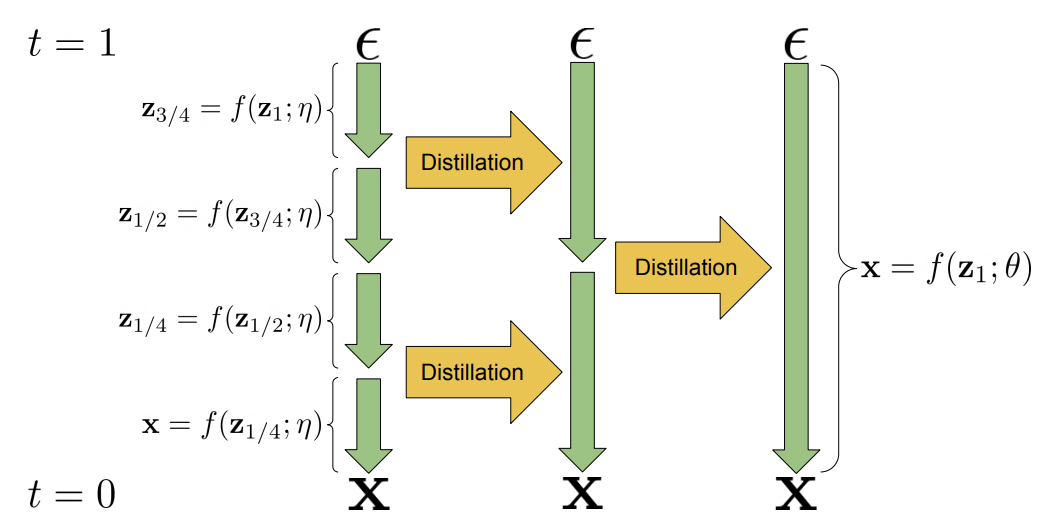
Progressive distillation trains a student one-step transition to match two consecutive teacher transitions:
\[f_\theta(z_t, t \to s) \approx f_\eta\left(f_\eta(z_t, t \to u), u \to s\right), \qquad t > u > s.\]Consistency Models
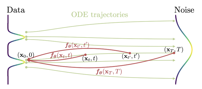
The key idea of Consistency Models is to learn a function whose output is consistent along the same probability-flow ODE trajectory. Instead of predicting only the next denoising step, the model maps noisy samples at different times to the same clean endpoint.
The consistency constraint is:
\[f_\theta(x_t,t) \approx f_\theta(x_{t^\prime},t^\prime), \qquad x_t,\;x_{t^\prime} \text{ on the same trajectory}.\]The practical question is how to obtain such paired points. Consistency Models use two main training setups: Consistency Distillation (CD) and Consistency Training (CT). The pair construction differs as follows:
\[\begin{cases} \text{Consistency Distillation (CD):} & x_{t^\prime} = \operatorname{ODESolver}(x_t, t \to t^\prime; s_\phi), \\ \text{Consistency Training (CT):} & x_t = \alpha_t x_0 + \sigma_t \epsilon,\quad x_{t^\prime} = \alpha_{t^\prime} x_0 + \sigma_{t^\prime} \epsilon. \end{cases}\]CD uses a pretrained score model $s_\phi$ and an ODE solver to move along the probability-flow trajectory, while CT constructs two noisy versions of the same clean sample using the same noise.
After training, one-step sampling is a single evaluation from terminal noise:
\[x_0 = f_\theta(x_T,T).\]Limitation
-
Unstable training. Consistency Models are highly sensitive to curriculum design, such as how the time discretization is scheduled and how difficult trajectory pairs are introduced during training.
-
Indirect training signal. The constraint $f_\theta(x_t,t) = f_\theta(x_{t^\prime},t^\prime)$ only says that two outputs should match. By itself, this admits trivial solutions, so practical training needs boundary conditions and other engineering tricks to make the shared output correspond to a real clean sample.
-
Dependence on diffusion teacher in CD. Consistency distillation still requires a pretrained diffusion or score model to construct reliable same-trajectory pairs.
CTM
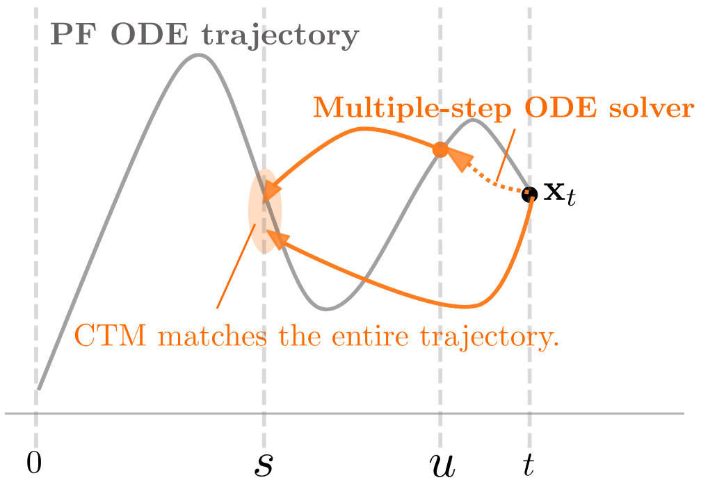
Consistency Trajectory Models (CTM) extend Consistency Models from endpoint consistency to trajectory consistency. Instead of only mapping a noisy point to the clean endpoint, CTM learns a transition map
\[G_\theta(x_t,t,s)\]that moves a sample from time $t$ to another time $s$ along the probability-flow ODE trajectory.
The trajectory consistency constraint is:
\[G_\theta(x_t,t,s) \approx G_\theta(G_\theta(x_t,t,u),u,s).\]That is, a direct jump from $t$ to $s$ should match a composed path through an intermediate time $u$.
CTM also has to handle special cases of the transition map. For example,
\[\begin{cases} G_\theta(x_t,t,t)=x_t, & \text{identity at the same time}, \\ G_\theta(x_t,t,0)\approx x_0, & \text{endpoint prediction}. \end{cases}\]After training, one-step sampling is:
\[x_0 = G_\theta(x_T,T,0).\]Because the target time $s$ is an input, the same model can also be used for multi-step sampling by composing shorter transitions. In that sense, CTM tries to learn the probability-flow ODE trajectory itself, not only the final endpoint.
Limitation
-
Additional constraints for special cases. CTM is more flexible than CM because it models transitions between arbitrary times, but that flexibility introduces boundary cases such as $s=t$ and $s=0$ that need to be handled by the parameterization and loss design.
-
Training stability. CTM still has an indirect training signal: the model is trained by making direct and composed paths agree, unlike MeanFlow’s velocity-regression-style objective.
-
Not self-contained. Strong practical performance requires an additional GAN component.
MeanFlow
The key idea of MeanFlow is to learn the average displacement over a time interval, rather than the instantaneous velocity at each time. Flow Matching learns a local velocity field $v(x_t,t)$ and then integrates it with an ODE solver. MeanFlow asks whether the model can learn the interval-level velocity directly.
The average velocity is defined as:
\[u(z_t,r,t) = \frac{1}{t-r} \int_r^t v(z_\tau,\tau)\,d\tau.\]The training signal comes from the MeanFlow identity, which connects this average velocity to the instantaneous velocity:
\[v(z_t,t) = \partial_z u \cdot v + \partial_t u.\]The derivative term is computed with a Jacobian-vector product (JVP), so the method can train the average-velocity model with a regression-style objective rather than a trajectory-consistency constraint.
After training, one-step sampling applies the learned average displacement over the full interval:
\[x_1 = \epsilon + u_\theta(\epsilon,0,1).\]Limitation
- Additional constraint for the special case. When the interval collapses, MeanFlow needs the average velocity to match the instantaneous velocity:
DMD
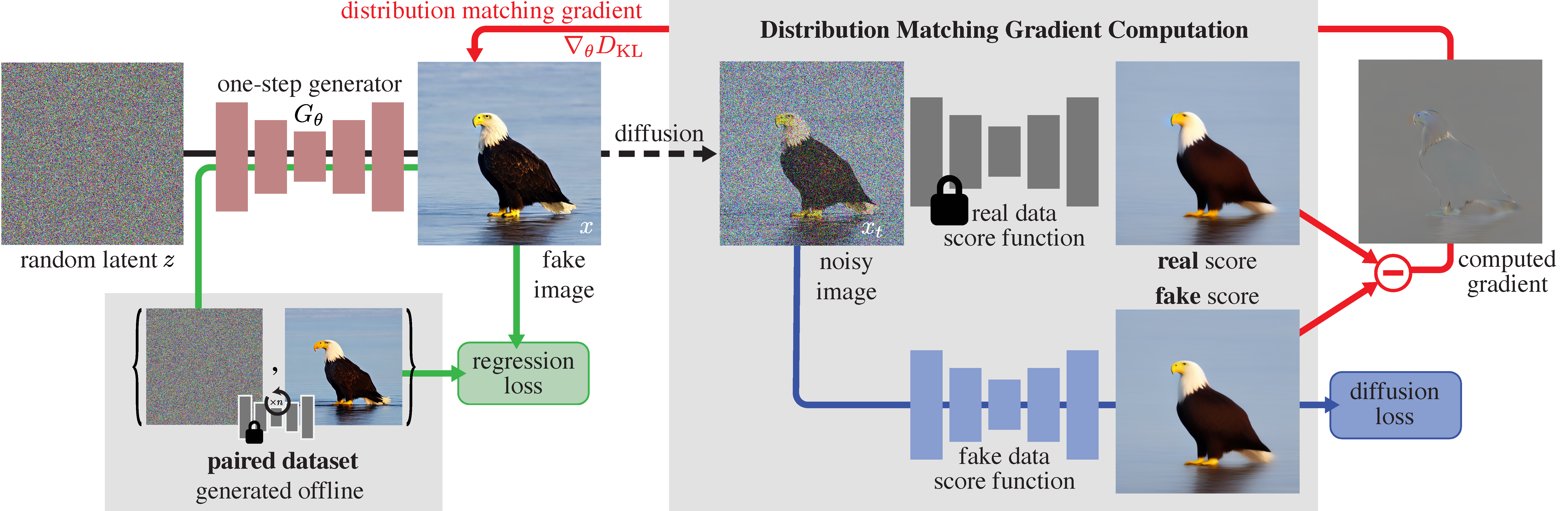
The key idea of Distribution Matching Distillation (DMD) is to train a one-step generator by directly matching the generated distribution to the data distribution. Instead of enforcing agreement along an ODE trajectory, DMD minimizes a KL divergence between the noised fake distribution and the noised real distribution:
\[\int_0^T w(t)\, D_{\mathrm{KL}}\!\left(q_t^{\mathrm{fake}} \,\|\, p_t^{\mathrm{real}}\right)\,dt.\]The important observation is that the gradient of this KL objective can be expressed using score functions:
\[\nabla_\theta \int_0^T w(t)\, D_{\mathrm{KL}}\!\left(q_t^{\mathrm{fake}} \,\|\, p_t^{\mathrm{real}}\right)\,dt \approx \int_0^T w'(t)\, \mathbb{E}_{\hat{x}_t} \left[ \epsilon_{\mathrm{real}}(\hat{x}_t,t) - \epsilon_{\mathrm{fake}}(\hat{x}_t,t) \right] \frac{\partial \hat{x}_t}{\partial \theta} \,dt.\]Here, the real score and fake score tell the generator how the fake distribution should move relative to the real distribution. After training, sampling is simply a single generator forward pass:
\[\hat{x}_0 = g_\theta(\epsilon), \qquad \epsilon \sim p_\epsilon.\]Limitation
-
Not self-contained. DMD requires a pretrained diffusion model to provide the score signal, and the one-step generator also needs a reasonably good initialization.
-
Heavy overhead before training. The method requires extra data-generation work, such as constructing paired noise-image data for distillation.
Comparing One-step Methods
| Method | Objective Type | ODE Dep. | Self-Contained |
|---|---|---|---|
| Diffusion Models | Regression | – | Yes |
| Consistency Models | Consistency constraint | Yes | Partial |
| CTM | Consistency constraint | Yes | Partial |
| MeanFlow | Regression (velocity) | Yes | Yes |
| DMD | Regression (KL-divergence) | No | No |
One thing I want to highlight from this table is the objective type. Consistency-based objectives are elegant, but the supervision is indirect: the model is asked to make two paths or two time points agree. Regression-style objectives are often easier to reason about and can be more stable in practice because they provide a more explicit target. This is somewhat orthogonal to the main topic of one-step generation, but it matters when comparing these methods as training recipes.
This is one reason MeanFlow and DMD are interesting in this list. MeanFlow turns flow learning into regression on an average velocity, while DMD turns distribution matching into a score-based regression signal. They are not free of assumptions, but their objectives are closer to direct regression than pure consistency constraints.
The remaining question is then not simply “can we generate in one step?” These methods already show several ways to do that. The more useful question is what kind of training signal makes one-step generation stable, self-contained, and less dependent on an inference-time trajectory or a pretrained diffusion teacher.
Drifting Models
Training-Time Distribution Evolution
Drifting Models take a different perspective on where the generative dynamics happen. In diffusion and flow models, the generated distribution evolves along pseudo-time while sampling. In Drifting Models, the generated distribution evolves during training.
 |
|---|
| Drifting Models shift the distribution evolution from inference-time sampling to training-time updates. |
Method
Drift
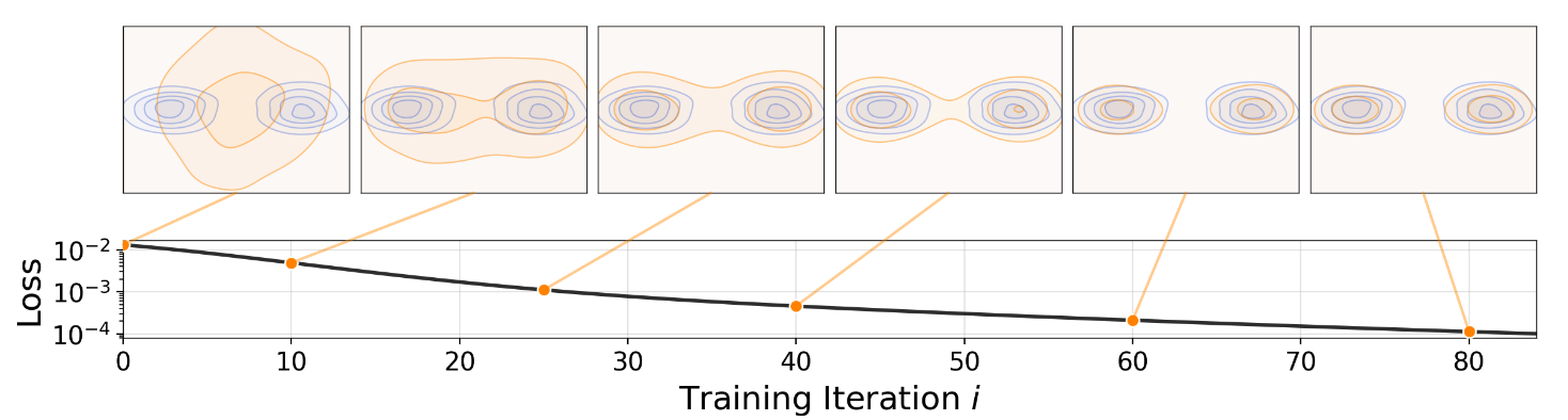
Suppose the generator at training step $i$ is $f_i$. For a fixed noise sample $\epsilon$, the generated point is $x_i = f_i(\epsilon)$. After one update, the generator becomes $f_{i+1}$ and the same noise maps to $x_{i+1} = f_{i+1}(\epsilon)$. The difference
\[\Delta x_i = f_{i+1}(\epsilon) - f_i(\epsilon)\]is the sample’s training-induced movement, which is why the method is called “drifting.” Since parameter updates already move generated samples during training, Drifting Models make this movement explicit and govern it with a drift field $V_{p,q}$, where $p$ is the data distribution and $q$ is the current model distribution.
Drift Field
The drift field $V_{p,q}(x)$ determines how a generated sample should move when the current model distribution is $q$ and the target distribution is $p$. The desired equilibrium is clear: when $p=q$, samples should stop drifting. To encode this, the field is designed to be anti-symmetric:
\[V_{p,q}(x) = -V_{q,p}(x).\]If $p=q$, anti-symmetry implies $V_{p,q}(x)=0$. The converse is more delicate. A zero drift field does not generally guarantee that $p=q$, so the theory relies on expressive kernels and additional identifiability assumptions. This is one of the important gaps in the method.
Training Objective
The training objective is derived from the fixed-point relation at equilibrium:
\[f_{\hat{\theta}}(\epsilon) = f_{\hat{\theta}}(\epsilon) + V_{p,q_{\hat{\theta}}}\!\left(f_{\hat{\theta}}(\epsilon)\right).\]Drifting Models turn this relation into a stop-gradient regression target:
\[L(\theta; \textcolor{#B509AC}{q_\theta}) = \mathbb{E}_{\epsilon} \left[ \left\| \underbrace{f_\theta(\epsilon)}_{\text{prediction}} - \underbrace{ \operatorname{sg} \left( f_\theta(\epsilon) + V_{p,\textcolor{#B509AC}{q_\theta}}(f_\theta(\epsilon)) \right) }_{\text{frozen target}} \right\|^2 \right].\]The important part is the dependence on $\textcolor{#B509AC}{q_\theta}$. The objective changes with the current generated distribution, so training is not just fitting a pre-defined target field; it repeatedly updates the target according to the model’s own distribution.
Drifting Field Design
The drift field is built from an attraction-repulsion interaction. For a generated point $x$, positive samples $y^+$ come from the data distribution and negative samples $y^-$ come from the generated distribution. A kernel $k(x,y)$ measures similarity, and the resulting drift has the form of an attraction toward real samples and a repulsion away from generated samples:
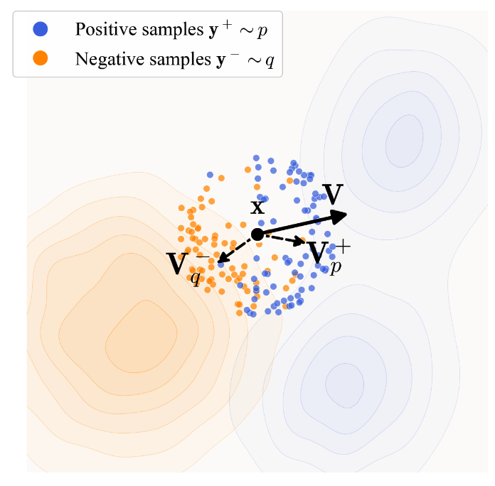
Formally, the drifting field is defined as
\[V_{p,q}(x) \propto \mathbb{E}_{y^+ \sim p,\; y^- \sim q} \left[ k(x,y^+) k(x,y^-)(y^+ - y^-) \right].\]This construction satisfies the anti-symmetry condition $V_{p,q}=-V_{q,p}$. The form is close in spirit to contrastive learning: similar real samples pull the generated point, while similar fake samples provide repulsion.
Implementation Details
Two practical details matter for applying the drift objective to image generation: feature-space drift and CFG-conditioned sampling.
Encoder-Based Drift
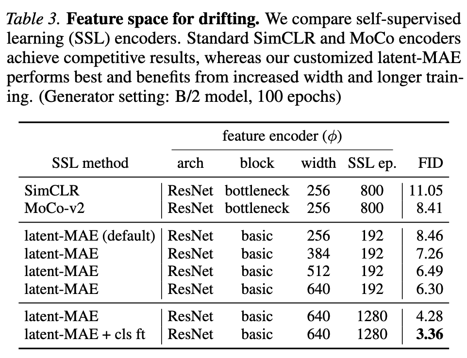
Doing the attraction-repulsion computation directly in raw pixel space is not enough. Pixel distances do not capture semantic similarity well in high-dimensional image domains, so the practical version computes similarity in feature space using a frozen self-supervised encoder $\phi$, such as MoCo, SimCLR, or latent-MAE features. In effect, the kernel becomes
\[k_\phi(x,y) = k(\phi(x),\phi(y)).\]The generator can still output pixels or latents, and the encoder is used only during training to construct the drift target. At inference time, the encoder is not evaluated. This is why I would describe Drifting Models as not ODE-dependent, but not completely assumption-free: they remove the diffusion teacher and inference-time trajectory, but introduce a strong dependence on representation and kernel design.
Classifier-Free Guidance
For conditional generation, CFG is introduced by changing how the positive and negative samples are drawn:
\[\begin{aligned} y^+ &\sim p_{\mathrm{data}}(\cdot \mid c), \\ y^- &\sim \tilde{q}(\cdot \mid c) = (1-\gamma)q_\theta(\cdot \mid c) + \gamma p_{\mathrm{data}}(\cdot \mid \phi_{\mathrm{null}}), \end{aligned}\]$\phi_{\mathrm{null}}$ denotes the null condition. During training, the drift field constructed from these positive and negative samples is used to train the $\gamma$-conditioned generator $f_\theta(\epsilon,c,\gamma)$. During sampling, the drift field is not evaluated. The trained generator directly takes the condition and guidance scale:
\[x = f_\theta(\epsilon,c,\gamma), \qquad \epsilon \sim p_\epsilon.\]So CFG is not applied by mixing two predictions at every denoising step, as in diffusion sampling. It is learned during training and exposed as an input to the one-step generator.
Results
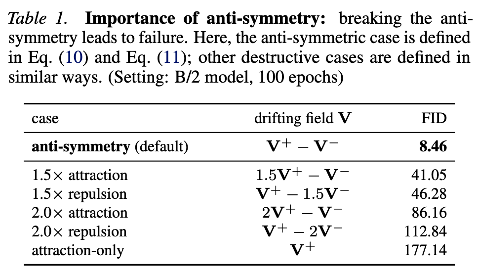
Importance of Anti-Symmetry
The anti-symmetric attraction-repulsion structure is not cosmetic. When the balance is broken, FID degrades sharply, which suggests that the field design is central to the method.
 |
|---|
| Breaking the anti-symmetric attraction-repulsion design substantially degrades FID. |
Ablations on Encoders
The feature encoder is another major factor. The ablation shows that representation choice has a large effect on FID, reinforcing that Drifting Models depend strongly on the feature space used to compute the kernel.
 |
|---|
| The feature encoder choice is a major part of the method’s empirical behavior. |
Limitation
-
Theoretical gap. A vanishing drift field, $V \to 0$, does not by itself guarantee $p=q$; the identifiability argument remains heuristic.
-
Kernel and representation dependency. The field is computed through $k(\phi(x),\phi(y))$, so performance depends heavily on the encoder and kernel design.
-
Design optimality is not guaranteed. The kernel, drifting field, and architecture are still design choices with room for improvement.
-
Scalability is still unverified. The presented setting does not yet cover generation beyond $256 \times 256$ or text conditioning, and the contrastive-like objective benefits from large batch sizes.
Positioning
| Method | Objective Type | ODE Dep. | Self-Contained |
|---|---|---|---|
| Diffusion Models | Regression | – | Yes |
| Consistency Models | Consistency constraint | Yes | Partial |
| CTM | Consistency constraint | Yes | Partial |
| MeanFlow | Regression (velocity) | Yes | Yes |
| DMD | Regression (KL-divergence) | No | No |
| Drifting Models | Regression (drift) | No | Partial |
References
- Luhman and Luhman, Knowledge Distillation in Iterative Generative Models for Improved Sampling Speed (2021).
- Salimans and Ho, Progressive Distillation for Fast Sampling of Diffusion Models (ICLR 2022).
- Song et al., Consistency Models (ICML 2023).
- Kim et al., Consistency Trajectory Models: Learning Probability Flow ODE Trajectory of Diffusion (ICLR 2024).
- Geng et al., Mean Flows for One-Step Generative Modeling (NeurIPS 2025).
- Yin et al., One-step Diffusion with Distribution Matching Distillation (CVPR 2024).
- Deng et al., Generative Modeling via Drifting (arXiv:2602.04770).