Learning to tokenize (2): How LH-Net works
LH-Net and H-Net#
The previous post explored the motivation behind H-Net and what it can do. In this post, we turn to Dynamic Chunking for End-to-End Hierarchical Sequence Modeling[1] to understand how it works.
Following Cartesia’s distinction ↗, we call the original model LH-Net, where “L” stands for “lazy” or “lookahead.” Although Cartesia has not disclosed the full architectural details of the updated H-Net, it highlights a key difference: LH-Net draws a boundary only after seeing the start of the next chunk. This gives it more context for chunking, but, according to Cartesia, hurts next-byte prediction. While LH-Net differs from the H-Net discussed in the previous post, studying it provides a technical foundation for understanding hierarchical sequence modeling.
A lens for understanding sequence modeling#
We can view tokenization and learned compression methods through a shared frame: encode raw inputs into a shorter sequence, process it with a main network, and decode the result into raw-level predictions. They differ in how they construct these compressed representations—and which parts of this process are learned jointly with the main network. Keeping this picture in mind, we will first look at earlier approaches, then examine how LH-Net learns to form and use these representations.
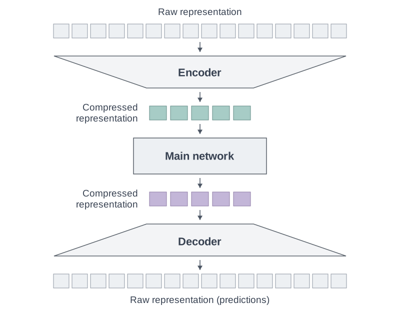
Viewed through this lens, BPE and the prior approaches discussed in the paper differ in how they construct compressed representations and choose their boundaries. The limitations below follow the paper’s discussion.
| Approach | How compression works | Limitation |
|---|---|---|
| BPE[3] | Merge bytes into vocabulary tokens. | Segmentation stays fixed during language-model training. |
| Direct byte modeling (MambaByte[4]) | — | Processing the full byte sequence remains costly. |
| Fixed-size chunking (Hourglass[5], MegaByte[6]) | Encode each group of | Boundaries do not adapt to content. |
| Heuristic chunking (SpaceByte[7], BLT[8]) | Form chunks using delimiter or entropy rules. | The boundary-selection rule may not align with the main objective. |
| End-to-end chunking (DPT’s Gumbel variant[9]) | Learn chunk boundaries jointly with next-token prediction. | Training instability limits scaling and deeper hierarchies. |
Note. Entropy rules place boundaries where uncertainty about the next byte is high or rises sharply.
LH-Net follows the same end-to-end direction as the last approach, with architectural and training changes designed to make learned chunking stable and scalable across model sizes and hierarchy levels.
LH-Net architecture overview#
LH-Net follows an encoder → chunking layer → main network → dechunking layer → decoder structure. During autoregressive generation, the encoder and decoder run at every byte, while the main network advances only when a new chunk boundary is selected.
Crucially, the main network can itself be another LH-Net, allowing the same structure to repeat across multiple levels of compression. The paper’s Figure 1 shows a two-stage example. For simplicity, this post focuses on a single-stage architecture with one encoder, one main network, and one decoder.
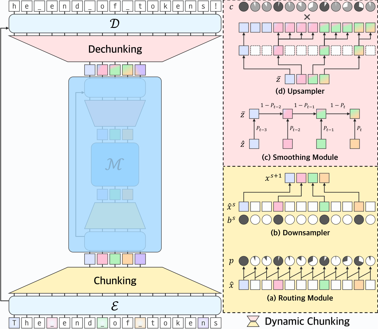
The architecture and its learning objective can be understood through the following principles:
- Keep the encoder and decoder efficient. Since the encoder and decoder process long, uncompressed sequences, they use efficient state space models: four Mamba-2 layers in each encoder and decoder.
- Preserve fine-grained information for the decoder. The encoder passes fine-grained information through residual connections.
- Concentrate compute and model capacity in the main network. The main network operates on a shorter sequence of richer representations. The encoder builds these representations, and the chunking layer reduces the sequence length.
- Use next-byte prediction as the main learning signal, including for chunking. Learn chunk boundaries that support next-byte prediction, without explicit boundary supervision.
Dynamic chunking#
In LH-Net, the encoder preserves sequence length so that the model can decide where to place chunk boundaries before compression. There are no ground-truth boundary labels; instead, boundary decisions are learned to improve next-byte prediction.
The chunking layer uses a routing module to determine boundaries and a downsampler to construct compressed representations. The dechunking layer uses a smoothing module to support stable boundary learning and an upsampler to restore the original sequence length. The decoder then processes these full-length representations to predict the next byte at each position.
Chunking layer#
For a single hierarchy level, the encoder first produces a representation at every input position, then the chunking layer returns a shorter sequence and routing scores:
Routing module#
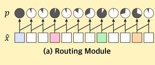
The routing module builds on the intuition that meaningful boundaries tend to occur where context or meaning shifts. Each encoder output
Here,
Downsampler#
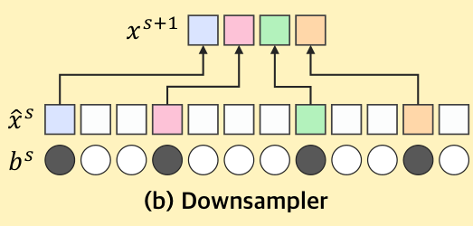
The downsampler constructs a compressed sequence using the boundaries selected by the routing module. LH-Net selects encoder outputs at boundary positions, rather than pooling the representations within each chunk. The same selection is applied to the routing scores: retaining only the boundary positions from
Dechunking layer#
The dechunking layer takes the main network output
Smoothing module#
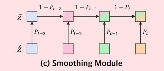
The smoothing module blends the main network’s output
Here,
The smoothing module serves three roles:
- Boundary learning: provide a differentiable path from the prediction loss to the routing scores.
- Error correction: soften the effect of uncertain boundaries by incorporating information from preceding chunks.
- Training stability: reduce early commitment to suboptimal chunking patterns.
Upsampler#
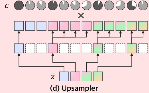
The upsampler restores the original sequence length by repeating each smoothed chunk representation until the next boundary:
It then weights the result by the router’s confidence in the current decision,
Here,
The inner product measures how the loss changes as the scale of
Training objective#
LH-Net’s objective is next-byte prediction with compression regularization. The prediction loss provides the main learning signal for the entire model, including chunking, while the ratio loss encourages each stage to meet its target compression ratio.
for
Interpreting the ratio loss as a chi-square divergence
With target boundary rate
If
where the second term is the chi-square divergence of the actual boundary rate from the target rate. The ratio loss replaces one factor of
References#
-
Cartesia Research, From tokens to bytes I: Scaling hierarchical networks (2026) ↗
-
Junxiong Wang et al., MambaByte: Token-free Selective State Space Model (2024) ↗
-
Lili Yu et al., MEGABYTE: Predicting Million-byte Sequences with Multiscale Transformers (2023) ↗
-
Kevin Slagle, SpaceByte: Towards Deleting Tokenization from Large Language Modeling (2024) ↗
-
Artidoro Pagnoni et al., Byte Latent Transformer: Patches Scale Better Than Tokens (2024) ↗
-
Piotr Nawrot et al., Efficient Transformers with Dynamic Token Pooling (ACL 2023) ↗